Optimizers Are Memory: A Visual Guide from SGD to AdamW
Optimizers Are Memory: A Visual Guide from SGD to AdamW
Most deep learning code eventually arrives at a line that looks like this:
optimizer = torch.optim.AdamW(model.parameters(), lr=3e-4)
It is easy to treat this as plumbing. The model is the interesting part. The loss is the mathematical part. Backpropagation is the magical part. The optimizer is just the thing we import so training can begin.
But that one line decides how every parameter in the model moves.
Backpropagation gives us gradients. The optimizer decides what to do with them.
A gradient answers a local question:
If I nudge this parameter right now, which direction makes the loss go down fastest?
An optimizer answers a slightly richer question:
Given what I know about this gradient, and what I remember from previous gradients, how should I update the parameter?
That distinction is the whole post.
In this article, we will build several optimizers from scratch and visualize how they behave:
- SGD follows the current gradient.
- Momentum remembers direction.
- RMSProp remembers gradient scale.
- Adam remembers both direction and scale.
- AdamW uses Adam’s memory but decouples weight decay from the adaptive gradient update.
The central idea is:
Optimizers are memory mechanisms.
Some remember nothing. Some remember where gradients have been pointing. Some remember how large gradients have been. Adam remembers both. AdamW adds one more important idea: regularization should not be distorted by Adam’s adaptive scaling.
This is not a benchmark post. We are not trying to prove that one optimizer is universally best. Instead, we will create small controlled worlds where each optimizer’s behavior becomes visible.
The goal is to understand why these optimizers exist.
1. SGD: no memory
The simplest optimizer is gradient descent.
If the parameter vector is (w_t), the gradient is (g_t), and the learning rate is (\eta), then the update is:
\[w_{t+1} = w_t - \eta g_t\]That is the whole algorithm.
In code, SGD is almost embarrassingly simple:
class SGD:
    def __init__(self, lr):
        self.lr = lr

    def step(self, params, grads):
        for p, g in zip(params, grads):
            p -= self.lr * g
SGD has no optimizer state. It does not remember previous gradients. It does not remember whether the last update went well. It simply looks at the current gradient and steps in the opposite direction.
That sounds naive, but on a friendly loss surface it is exactly what we want.
Consider a simple round bowl:
\[f(x, y) = \frac{1}{2}(x^2 + y^2)\]The gradient is:
\[\nabla f(x, y) = [x, y]\]At every point, the gradient points directly away from the minimum. Following the negative gradient moves us cleanly toward the center.
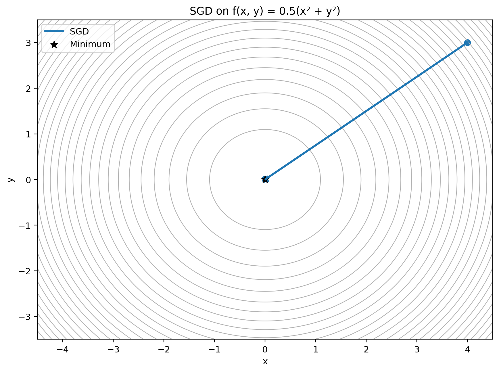
On a round bowl, the current gradient is a reliable guide. SGD does not need memory when the landscape is this friendly.
This is the best possible case for SGD. The loss is smooth, symmetric, and equally curved in every direction. The current gradient contains enough information to make good progress.
The lesson is not that SGD is bad.
The lesson is:
SGD works when the current gradient is a good guide.
Problems start when the current gradient is locally correct but globally inefficient.
2. When SGD zig-zags
Now consider a slightly less friendly loss:
\[f(x, y) = \frac{1}{2}(x^2 + 50y^2)\]The gradient is:
\[\nabla f(x, y) = [x, 50y]\]This is still a convex quadratic. There are no local minima. There is no neural network weirdness. The optimum is still at the origin.
But the curvature is very different in the two directions.
The (y)-direction is steep. The (x)-direction is shallow. The result is a narrow valley.
In this kind of landscape, the steepest local direction often points across the valley, not along it. SGD sees a large gradient in the steep direction, steps across the valley, then sees a large gradient pointing back the other way.
It zig-zags.
The problem is not that the gradient is wrong. The gradient is locally correct. The problem is that SGD has no memory. It does not notice that the sideways component keeps changing sign while the useful direction remains consistent.
That gives us the motivation for momentum.
3. Momentum: direction memory
Momentum adds a velocity vector.
Instead of using only the current gradient, we maintain a running direction:
\[v_t = \beta v_{t-1} + g_t\]Then we update parameters using that velocity:
\[w_{t+1} = w_t - \eta v_t\]Here, (\beta) controls how much past gradient information we keep. A common value is (0.9).
The code is still simple:
class Momentum:
    def __init__(self, lr, beta=0.9):
        self.lr = lr
        self.beta = beta
        self.velocity = None

    def step(self, params, grads):
        if self.velocity is None:
            self.velocity = [np.zeros_like(p) for p in params]

        for i, (p, g) in enumerate(zip(params, grads)):
            self.velocity[i] = self.beta * self.velocity[i] + g
            p -= self.lr * self.velocity[i]
Momentum is often described as “accelerating” gradient descent. That is true, but incomplete.
A better mental model is:
Momentum is a low-pass filter over gradients.
If gradients keep pointing in the same direction, momentum accumulates them. If gradients keep flipping direction, momentum partially cancels them.
That is exactly what we want in a narrow valley.
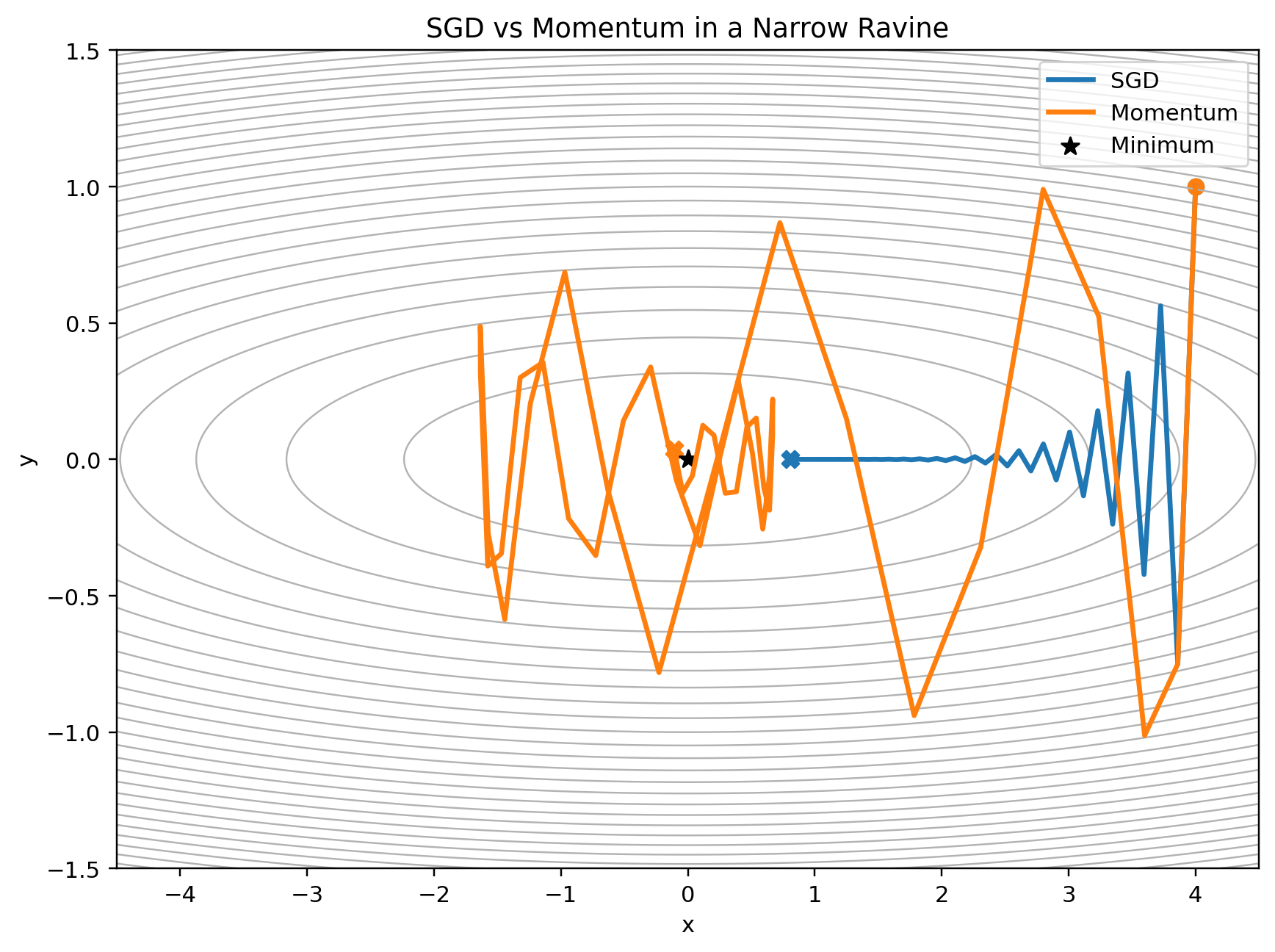
SGD keeps reacting to the latest sideways gradient. Momentum remembers the directions that persist and damps directions that flip.
In the steep direction, SGD alternates back and forth. Momentum sees that alternation and smooths it out. In the shallow direction, gradients are more consistent, so momentum builds speed.
This is the first kind of optimizer memory:
Momentum remembers direction.
It does not know anything about the scale of each parameter’s gradients. It just remembers where gradients have been pointing.
Sometimes that is enough. Sometimes it is not.
4. RMSProp: scale memory
A single global learning rate can be awkward.
Suppose one parameter regularly receives large gradients while another parameter regularly receives small gradients. If the learning rate is large enough for the small-gradient parameter, it may be too large for the high-gradient parameter. If it is small enough for the high-gradient parameter, progress in the low-gradient direction may be painfully slow.
RMSProp addresses this by keeping a running average of squared gradients:
\[s_t = \beta s_{t-1} + (1 - \beta)g_t^2\]Then it divides the gradient by the root of this running average:
\[w_{t+1} = w_t - \eta \frac{g_t}{\sqrt{s_t} + \epsilon}\]The square and square root are applied elementwise.
The idea is:
If a coordinate has consistently large gradients, reduce its effective step size.
If a coordinate has consistently small gradients, allow relatively larger steps.
In code:
class RMSProp:
    def __init__(self, lr, beta=0.9, eps=1e-8):
        self.lr = lr
        self.beta = beta
        self.eps = eps
        self.sq_avg = None

    def step(self, params, grads):
        if self.sq_avg is None:
            self.sq_avg = [np.zeros_like(p) for p in params]

        for i, (p, g) in enumerate(zip(params, grads)):
            self.sq_avg[i] = self.beta * self.sq_avg[i] + (1 - self.beta) * (g ** 2)
            p -= self.lr * g / (np.sqrt(self.sq_avg[i]) + self.eps)
RMSProp is not remembering direction. It is remembering scale.
To visualize this, we can use a loss where the two coordinates have very different gradient magnitudes:
\[f(x, y) = \frac{1}{2}(0.1x^2 + 50y^2)\]The gradient is:
\[\nabla f(x, y) = [0.1x, 50y]\]The (y)-coordinate produces much larger gradients than the (x)-coordinate. SGD has one learning rate for both. RMSProp adapts the effective learning rate per coordinate.
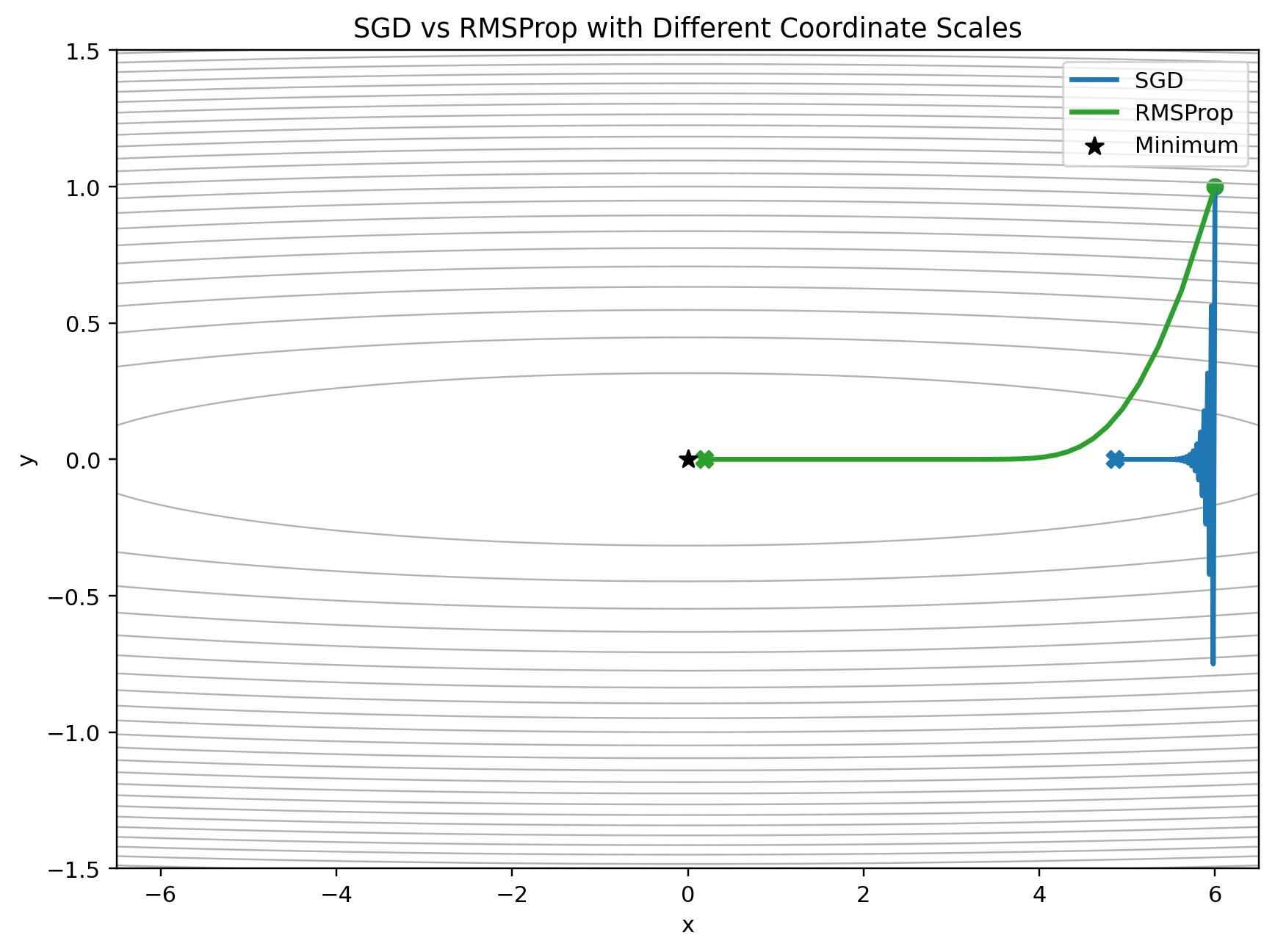
RMSProp remembers how large each coordinate’s gradients have been. Coordinates with consistently large gradients get smaller effective steps.
This is the second kind of optimizer memory:
RMSProp remembers gradient scale.
That makes it useful when different parameters live on different gradient scales.
But RMSProp does not remember direction in the same way momentum does. It rescales gradients, but it does not smooth them into a velocity.
So the natural question is: can we remember both?
5. Adam: direction memory plus scale memory
Adam combines the two memories.
It keeps a running average of gradients:
\[m_t = \beta_1 m_{t-1} + (1 - \beta_1)g_t\]and a running average of squared gradients:
\[v_t = \beta_2 v_{t-1} + (1 - \beta_2)g_t^2\]The first moment, (m_t), behaves like momentum. It remembers direction.
The second moment, (v_t), behaves like RMSProp. It remembers scale.
Adam then updates parameters with:
\[w_{t+1} = w_t - \eta \frac{\hat{m}_t}{\sqrt{\hat{v}_t} + \epsilon}\]where $\hat{m}_t$ and $\hat{v}_t$ are bias-corrected estimates. We will discuss those in the next section.
A compact implementation looks like this:
class Adam:
    def __init__(self, lr, beta1=0.9, beta2=0.999, eps=1e-8):
        self.lr = lr
        self.beta1 = beta1
        self.beta2 = beta2
        self.eps = eps
        self.t = 0
        self.m = None
        self.v = None

    def step(self, params, grads):
        if self.m is None:
            self.m = [np.zeros_like(p) for p in params]
            self.v = [np.zeros_like(p) for p in params]

        self.t += 1

        for i, (p, g) in enumerate(zip(params, grads)):
            self.m[i] = self.beta1 * self.m[i] + (1 - self.beta1) * g
            self.v[i] = self.beta2 * self.v[i] + (1 - self.beta2) * (g ** 2)

            m_hat = self.m[i] / (1 - self.beta1 ** self.t)
            v_hat = self.v[i] / (1 - self.beta2 ** self.t)

            p -= self.lr * m_hat / (np.sqrt(v_hat) + self.eps)
Adam is popular because real training gradients are messy.
They are noisy because we train on minibatches. They are differently scaled because parameters play different roles. They are nonstationary because the model changes during training.
A useful toy version is a quadratic loss where we add noise to the gradient:
\[g_t = \nabla f(w_t) + \epsilon_t\]where:
\[\epsilon_t \sim \mathcal{N}(0, \sigma^2)\]Now the optimizer has to deal not only with curvature, but also with stochasticity.
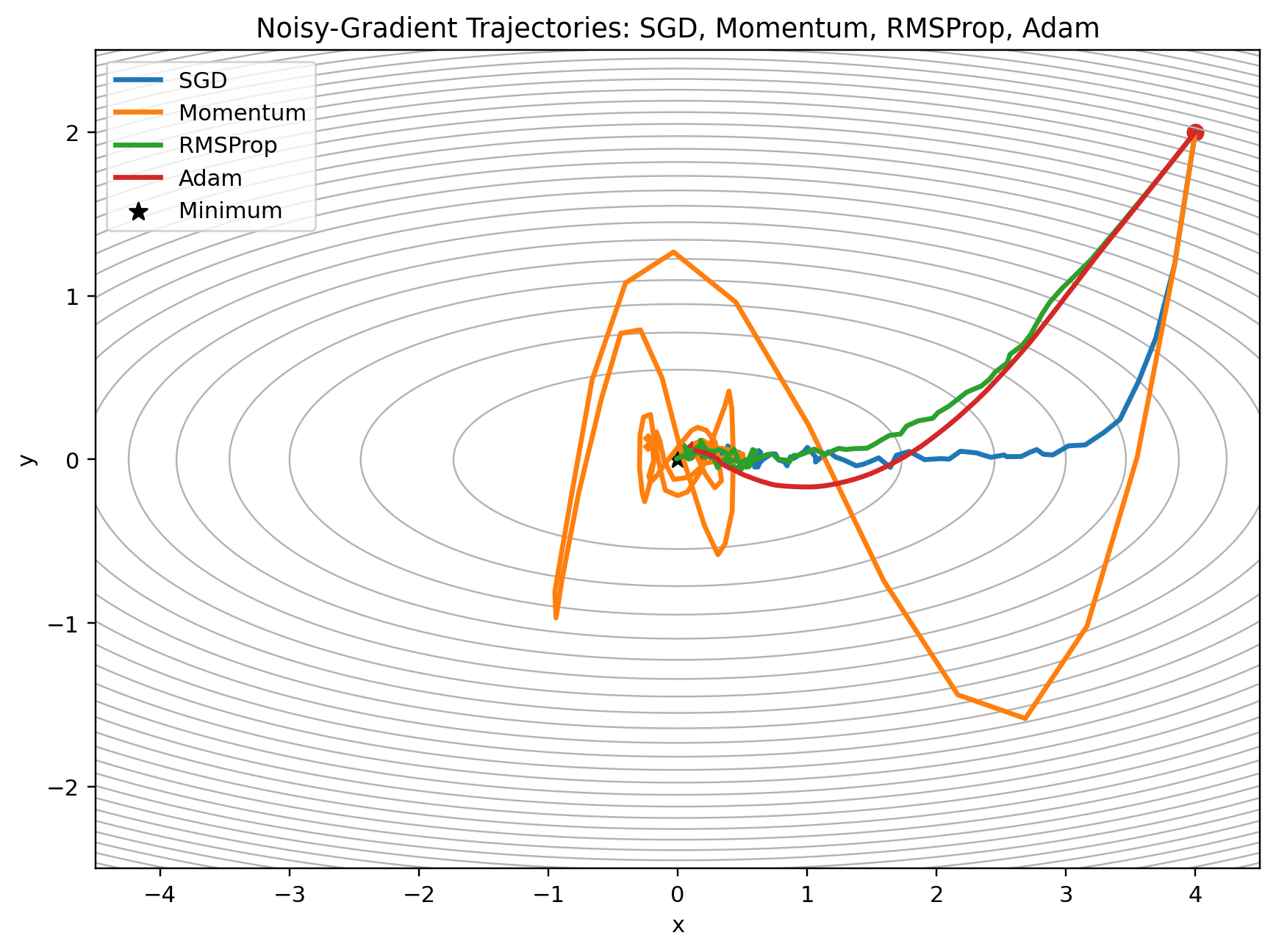
Adam combines direction memory and scale memory: the first moment smooths noisy directions, while the second moment rescales coordinates with consistently large gradients.
This is why Adam is often a strong default. It is not magic. It is forgiving because it carries more information forward from the past.
But there is an important detail hiding in the formula: bias correction.
6. Why bias correction exists
Adam initializes its moving averages at zero:
\[m_0 = 0\] \[v_0 = 0\]That creates a startup problem.
Suppose the gradient is always (1). If we use an exponential moving average with (\beta = 0.9), the first value is:
\[m_1 = 0.9 \cdot 0 + 0.1 \cdot 1 = 0.1\]But the true average of a constant sequence of ones should be (1), not (0.1).
The moving average is biased downward early because it started at zero.
Adam corrects this by computing:
\[\hat{m}_t = \frac{m_t}{1 - \beta_1^t}\]and:
\[\hat{v}_t = \frac{v_t}{1 - \beta_2^t}\]This correction matters most at the beginning of training.
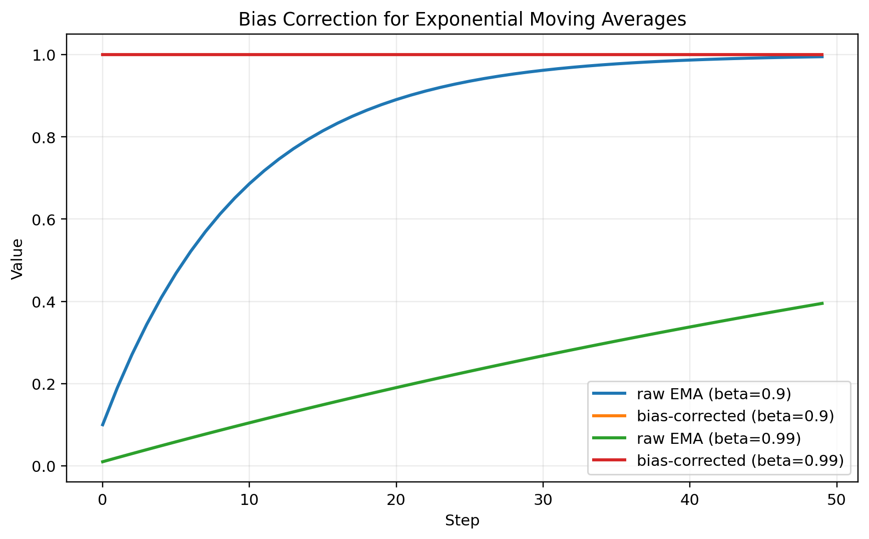
Moving averages initialized at zero underestimate early values. Bias correction removes this startup artifact.
Bias correction is easy to dismiss as a detail, but it is part of making Adam’s memory usable from the first few steps.
Without it, the optimizer’s early estimates are distorted by the arbitrary choice to initialize state at zero.
7. AdamW: decoupling weight decay
Adam gives us direction memory and scale memory. But there is one more issue: regularization.
In many models, we do not just want to minimize training loss. We also want to discourage weights from becoming unnecessarily large.
One common approach is L2 regularization, which adds a penalty to the loss:
\[L_{\text{total}}(w) = L_{\text{data}}(w) + \frac{\lambda}{2}\|w\|^2\]The gradient of the penalty is:
\[\lambda w\]So a common implementation adds the penalty directly to the gradient:
\[g_t \leftarrow g_t + \lambda w_t\]For plain SGD, this behaves like weight decay. The update becomes:
\[w_{t+1} = w_t - \eta(g_t + \lambda w_t)\]which can be rewritten as:
\[w_{t+1} = (1 - \eta \lambda)w_t - \eta g_t\]The weights shrink directly.
With Adam, however, adding (\lambda w_t) to the gradient means the regularization term goes through Adam’s adaptive machinery. It gets mixed into the first and second moments and divided by the adaptive denominator.
That means the regularization is no longer a simple direct shrinkage of the weights.
AdamW fixes this by decoupling weight decay from the gradient update:
\[w_{t+1} = w_t - \eta \cdot \text{AdamUpdate}(g_t) - \eta \lambda w_t\]The difference is subtle but important.
Adam with L2-style regularization:
grad = grad + weight_decay * param
adam_update(param, grad)
AdamW-style decoupled weight decay:
param = param * (1 - lr * weight_decay)
adam_update(param, grad)
In words:
Adam with L2 regularization regularizes through the adaptive gradient path.
AdamW decays weights directly.
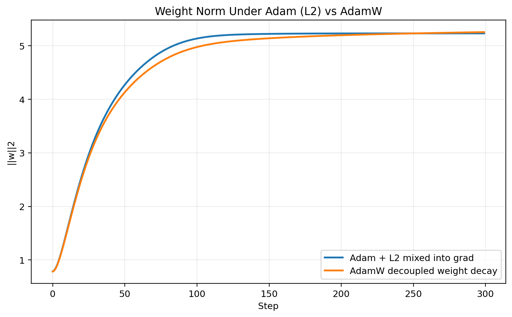
AdamW decays weights directly. Adam with L2 first mixes the penalty into the gradient, then sends it through Adam’s adaptive denominator.
This is why AdamW is not just “Adam with a different name.” It changes where regularization enters the update.
For modern neural networks, AdamW is often a better default than Adam with L2-style weight decay because the meaning of weight decay remains cleaner: shrink the weights directly, independent of the adaptive gradient scaling.
8. Sidebar: the memory cost of remembering
The phrase “optimizers are memory” is not just conceptual. It is literal.
For a model with (N) trainable parameters, different optimizers store different amounts of extra state.
| Optimizer | What it remembers | Extra optimizer state |
|---|---|---|
| SGD | nothing | (0) |
| Momentum | velocity | (N) |
| RMSProp | squared-gradient average | (N) |
| Adam | first moment and second moment | (2N) |
| AdamW | first moment and second moment | (2N) |
This is extra memory on top of the parameters and gradients.
For a tiny model, this does not matter much. For a model with billions of parameters, it matters a lot.
AdamW stores two extra tensors for every trainable parameter: one for the first moment and one for the second moment. In standard FP32 optimizer state, that can be a large part of training memory.
This is one reason large-scale training often cares about memory-efficient optimizer variants, optimizer sharding, and lower-precision optimizer states.
But for this post, the main lesson is simple:
The more an optimizer remembers, the more state it carries.
9. Linear regression sanity check
The toy surfaces above are designed for intuition. But we also want to verify that our from-scratch optimizers can train a real model.
We will use synthetic linear regression:
\[y = Xw + b + \epsilon\]This task is intentionally boring. That is the point.
Linear regression is simple enough that every reasonable optimizer should solve it. It is not a great way to show why Adam is interesting, but it is a good way to check that our implementations are not broken.
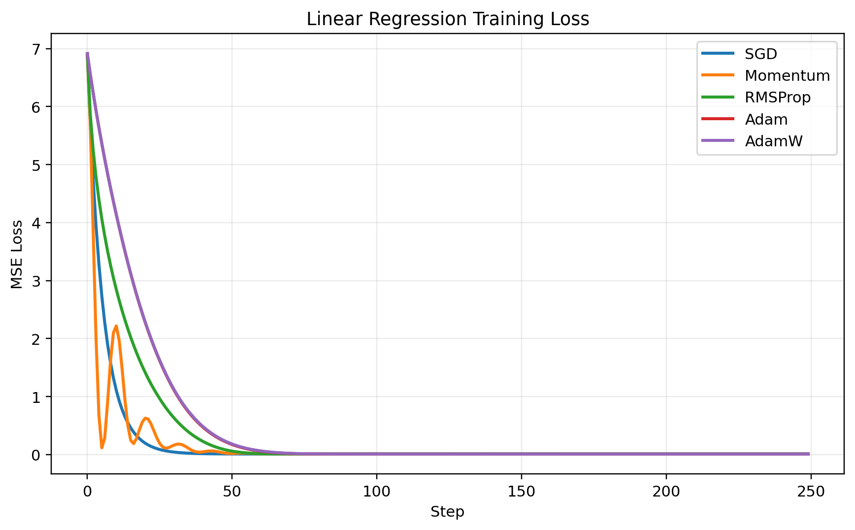
Linear regression is intentionally boring. It checks that every optimizer implementation can solve a simple differentiable problem.
This experiment also gives us a concrete way to count optimizer state.
For a linear model with (N) trainable parameters:
SGD state values: 0
Momentum state values: N
RMSProp state values: N
Adam state values: 2N
AdamW state values: 2N
This connects the implementation back to the thesis. Momentum, RMSProp, Adam, and AdamW differ not only in their equations, but also in the state they carry through training.
10. Tiny neural network on two moons
Toy loss surfaces are useful because we can see what is happening. But neural networks are not two-dimensional bowls.
So as a final bridge, we can train a tiny MLP on a two-moons classification task.
The model is intentionally small:
2 -> 32 -> 32 -> 1
With biases, this has:
Layer 1: 2*32 + 32 = 96
Layer 2: 32*32 + 32 = 1056
Output: 32*1 + 1 = 33
Total: 1185 parameters
The task is nonlinear, but still easy to visualize. We can plot the final decision boundary learned by different optimizers.
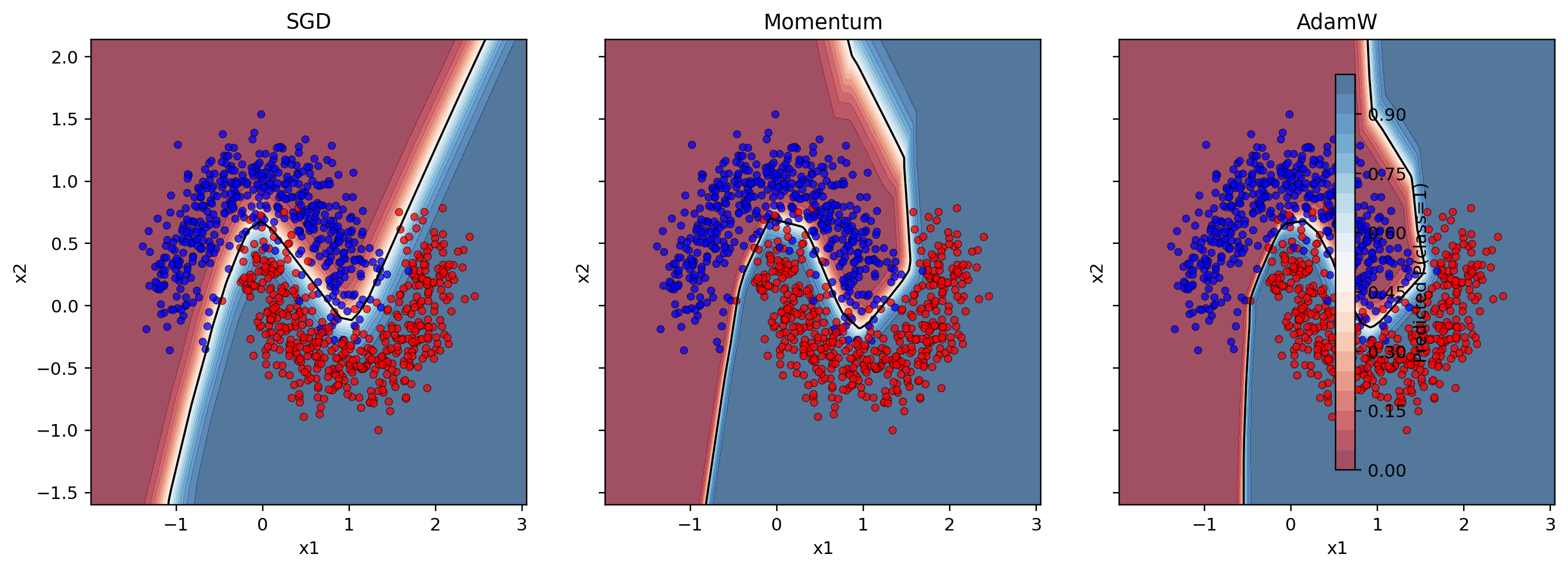
The two-moons task is small enough to visualize, but nonlinear enough that optimizer choice changes how quickly and cleanly the model finds a useful boundary.
This experiment should not be overinterpreted. It is not proof that one optimizer always generalizes better. It is just a small real model where optimizer behavior becomes visible.
The important connection is:
The same memories we saw in toy landscapes also shape neural-network training.
Momentum can smooth noisy directional changes. RMSProp-style scaling can help with uneven gradient magnitudes. AdamW combines adaptive optimization with cleaner weight decay.
11. Practical takeaways
Here is the practical version of the whole post.
SGD is the cleanest optimizer. It has no extra memory and follows the current gradient. It can work very well, especially with careful learning-rate schedules, but it can be sensitive to curvature and learning-rate choice.
Momentum adds direction memory. It is useful when gradients oscillate in some directions but remain consistent in others. It is not just “faster SGD”; it filters gradient history.
RMSProp adds scale memory. It tracks squared gradients and rescales updates per parameter. It is a stepping stone toward understanding Adam.
Adam combines direction memory and scale memory. It is often forgiving because it smooths noisy gradients and adapts to different coordinate scales.
AdamW keeps Adam’s memory but decouples weight decay from the adaptive gradient update. This makes regularization behavior cleaner and is one reason AdamW is widely used as a default in modern deep learning.
A reasonable default today is often:
optimizer = torch.optim.AdamW(model.parameters(), lr=3e-4, weight_decay=0.01)
But the optimizer does not remove the need to think.
The learning rate still matters. Weight decay still matters. Batch size still matters. Schedules still matter. The optimizer gives you an update rule, not a guarantee.
The better question is not:
Which optimizer is best?
The better question is:
What kind of memory does this training problem need?
12. What comes next
This post treated each optimizer as one global rule applied to all parameters.
Real training systems are more complicated.
A few natural next topics are:
- Learning-rate warmup and cosine decay: the learning rate itself changes over time.
- Nesterov momentum: a variant of momentum that looks ahead before computing the update.
- AdaGrad: an earlier adaptive method that accumulates squared gradients over the whole training run.
- Adafactor, Lion, Sophia, and 8-bit Adam: optimizer variants motivated by memory, speed, or large-model training.
- Parameter groups and layer-wise optimization: different parts of a model can use different learning rates, weight decay values, schedules, or even separate optimizers.
That last topic is especially important in fine-tuning. A pretrained backbone, a newly initialized head, embeddings, normalization parameters, and LoRA adapters may not all deserve the same optimization policy.
That is a different post.
For now, the core idea is enough:
Optimizers decide what to remember from the past.
SGD remembers nothing. Momentum remembers direction. RMSProp remembers scale. Adam remembers both. AdamW keeps Adam’s memories but handles weight decay separately.
Once you see optimizers this way, the formulas stop looking like arbitrary recipes.
They become different answers to the same question:
What information from previous gradients should influence the next step?
Reproducing the figures
The figures in this post were generated from scratch using small NumPy and PyTorch experiments.
To regenerate them:
python scripts/optimizers_memory/generate_all.py
The learning rates in these experiments are chosen for visual clarity and stable convergence. They should not be read as universal benchmark settings.